The Plane Wave

Expert Mode 1: The Plane Wave at the Double-Slit

We consider the propagation of a plane wave and its diffraction at a double-slit within the framework of scalar scattering theory. Here, we neglect its time dependence as we are interested in the steady-state condition.

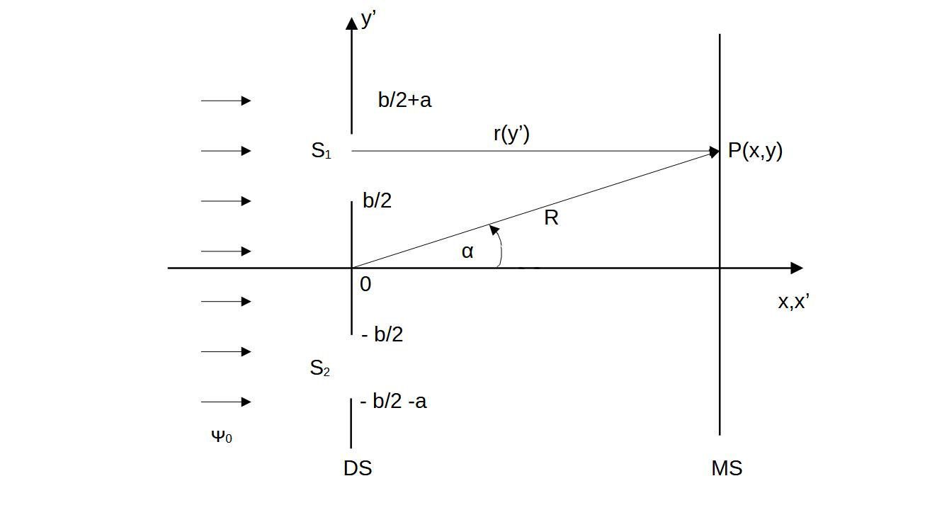
The Geometrical Setup (see Figure 1)
A plane wave $\Psi_0 = E_0 e^{ikx}$, generated by an ideal primary point source $S_p$ at $-\infty$ on the x-axis, propagates along the x-axis and hits a diaphragm with a double-slit (DS) at $x'=0$. The two slits each have width $a$ and are separated by an opaque barrier of width $b$. Far behind the double-slit (in the far field, $x \gg y$) is the measuring screen (MS), where we record the intensity of the field scattered at the double-slit at a point $P(x,y)$ under the observation angle $\alpha$.

Sources within the Kirchhoff Approximation
The incoming plane wave excites secondary sources in the two slit openings. Using the Heaviside step function $H$, these induced sources can be precisely formulated at the state level. For the upper slit $S_1$ and the lower slit $S_2$, they read in the Kirchhoff approximation:

\begin{align*} S_1(y') &= 2ik E_0 \cdot H\left(y' - \frac{b}{2}\right) \cdot H\left(\frac{b}{2} + a - y'\right) \\ S_2(y') &= 2ik E_0 \cdot H\left(-y' - \frac{b}{2}\right) \cdot H\left(\frac{b}{2} + a + y'\right) \end{align*}

The total source in the aperture plane is thus the simple sum $S(y') = S_1(y') + S_2(y')$ of both partial sources.

The Green's Function and the Field on the Screen
The field on the screen is calculated from the convolution integral of the sources with the Green's function

\begin{equation*} G(y, y') = \frac{e^{ikr(y')}}{4\pi R}, \end{equation*}

which describes the propagation of the scattered spherical waves. In the far field, we approximate the distance as $r(y') \approx R - y' \sin\alpha$.

The scattered field results in:

\begin{equation*} \Psi(\alpha) = \int_{-\infty}^{\infty} G(y,y') \cdot S(y') \, dy' \end{equation*}

This mathematical expression – the integral over the slit sources together with the specific Green's function – follows from the universally valid Huygens' principle. Due to the piecewise definition of the sources, the integral splits into two parts, giving us the asymptotic form of the wave on the screen:

\begin{equation*} \Psi(\alpha) = \Psi_1(\alpha) + \Psi_2(\alpha) = f(\alpha) \cdot E_0 \cdot \frac{e^{ikR}}{R} \end{equation*}

Scattering Amplitude and Superposition
The total scattering amplitude $f(\alpha)$ is the sum of the amplitudes of both slits: $f(\alpha) = f_1(\alpha) + f_2(\alpha)$. Integration over the respective slit widths yields:

\begin{align*} f_1(\alpha) &= \frac{ika}{2\pi} \cdot \frac{\sin \Gamma_a}{\Gamma_a} \cdot e^{-i\Gamma_+} \\ f_2(\alpha) &= \frac{ika}{2\pi} \cdot \frac{\sin \Gamma_a}{\Gamma_a} \cdot e^{+i\Gamma_+} \end{align*}

Here we use the abbreviations $\Gamma_{a,b} = \frac{k \cdot a,b}{2} \sin\alpha$ and $\Gamma_+ = \Gamma_a + \Gamma_b$.

Transition to Measurable Intensity
Up to this point, we have moved exclusively on the abstract state level. The interference of the two amplitudes is a pure superposition of complex phases. Only by taking the absolute square of the scattering amplitude do we obtain the intensity distribution $I_{DS}(\alpha)$ measurable on the screen in physical reality:

\begin{equation*} I_{DS}(\alpha) = |f(\alpha)|^2 = 4 \cdot I_S(\alpha) \cdot \cos^2\Gamma_+ \, . \end{equation*}

Here, $I_S(\alpha)$ is the intensity of a single slit of width $a$:

\begin{equation*} I_S(\alpha) = \left(\frac{ka}{2\pi}\right)^2 \cdot \frac{\sin^2\Gamma_a}{\Gamma_a^2}. \end{equation*}

The intensity of the double-slit is thus modulated by the term $\cos^2\Gamma_+$, which creates the typical interference fringes. However, the envelope of this fringe pattern is not simply the single-slit intensity, but exactly 4 times the single slit ($4 \cdot I_S(\alpha)$). This crucial factor of 4 is frequently missing in popular science presentations due to sloppy normalizations. Note that the Kirchhoff approximation used here is strictly valid only for small angles $\alpha$. In precisely this range, however, it agrees exceptionally well with actually measured intensities.

Literature Note:
Detailed integration steps and the grounded derivation of the Kirchhoff approximation via the Green's function can be found in: Rother, T.: Green's Functions in Classical Physics, Springer Int. Publ. AG, 2017.

For those interested in a rigorous solution to this scattering problem, see: Hönl, H., Maue A.W., Westphal, K.: Theorie der Beugung Handbuch der Physik Band 25/1, S. Flügge (Ed.). Springer, 1961.

---

Expert Mode 2: Interaction of a Linearly Polarized Plane Wave with a $\lambda/2$ Plate

We consider the basis states $|\varphi_1\rangle = |y\rangle = \begin{pmatrix} 0 \\ 1 \end{pmatrix}$ and $|\varphi_2\rangle = |z\rangle = \begin{pmatrix} 1 \\ 0 \end{pmatrix}$ with the orthogonality relation $\langle\varphi_i|\varphi_j\rangle = \delta_{ij}$. The initial states of two linearly polarized plane waves are defined as:

\begin{align*} |\psi_1\rangle &= \frac{e^{ikx}}{\sqrt{2}} |\varphi_1\rangle \\ |\psi_2\rangle &= e^{i\phi} \frac{e^{ikx}}{\sqrt{2}} |\varphi_2\rangle \end{align*}

Their intensities evaluate to $I_1 = \langle\psi_1|\psi_1\rangle = \frac{1}{2}$ and $I_2 = \langle\psi_2|\psi_2\rangle = \frac{1}{2}$. The total state is their superposition $|\psi\rangle = |\psi_1\rangle + |\psi_2\rangle$ with total intensity $I_g = \langle\psi|\psi\rangle = 1$. This superposition describes a linearly polarized plane wave propagating along the x-axis whose polarization plane at $\phi=0$ lies at an angle of $45^\circ$ to the positive z-axis.

Rotation by the $\lambda/2$ Plate
A $\lambda/2$ plate placed on the x-axis at point $x_w$ rotates the polarization plane by angle $\alpha_p$. In the new rotated coordinates $|\tilde{\varphi}_1\rangle$ and $|\tilde{\varphi}_2\rangle$, the state can be expressed via a coordinate transformation.

In the new coordinates, the transformed basis vectors read:

\begin{align*} |\tilde{\varphi}_1\rangle &= \begin{pmatrix} \cos\alpha_p \\ -\sin\alpha_p \end{pmatrix} \\ |\tilde{\varphi}_2\rangle &= \begin{pmatrix} \sin\alpha_p \\ \cos\alpha_p \end{pmatrix}, \end{align*}

which result from multiplying the old basis vectors by the rotation matrix

\begin{equation*} \hat{R} = \begin{pmatrix} -\sin\alpha_p & \cos\alpha_p \\ \cos\alpha_p & \sin\alpha_p \end{pmatrix} \end{equation*}

They satisfy the orthogonality relations $\langle\tilde{\varphi}_i|\tilde{\varphi}_j\rangle = \delta_{ij}$. Thus, the incoming partial fields can be expressed in the new coordinates as:

\begin{align*} |\tilde{\psi_1}\rangle &= \frac{e^{ikx}}{\sqrt{2}} \left( -\sin\alpha_p |\tilde{\varphi}_1\rangle + \cos\alpha_p |\tilde{\varphi}_2\rangle \right) \\ |\tilde{\psi_2}\rangle &= e^{i\phi} \frac{e^{ikx}}{\sqrt{2}} \left( \cos\alpha_p |\tilde{\varphi}_1\rangle + \sin\alpha_p |\tilde{\varphi}_2\rangle \right) \end{align*}

For the total field $|\tilde{\psi}\rangle = |\tilde{\psi_1}\rangle + |\tilde{\psi_2}\rangle$, addition in the new basis yields:

\begin{equation*} |\tilde{\psi}\rangle = \frac{e^{ikx}}{\sqrt{2}} \left[ \left(-\sin\alpha_p + e^{i\phi}\cos\alpha_p\right) |\tilde{\varphi}_1\rangle + \left(\cos\alpha_p + e^{i\phi}\sin\alpha_p\right) |\tilde{\varphi}_2\rangle \right] \end{equation*}

Again, total intensity satisfies $\langle\tilde{\psi}|\tilde{\psi}\rangle = 1$, meaning rotation of the polarization plane preserves intensity.

The Intensity Operator
A central element for determining measurable intensities is the intensity operator $\hat{I}$:

\begin{equation*} \hat{I} = \sum_{i=1}^4 p_i |\phi_i\rangle\langle\phi_i| \end{equation*}

This is formed from the sum of the dyadic products of the vectors

\begin{align*} |\phi_1\rangle &= -\sin\alpha_p |\tilde{\varphi}_1\rangle + \cos\alpha_p |\tilde{\varphi}_2\rangle \\ |\phi_2\rangle &= \cos\alpha_p |\tilde{\varphi}_1\rangle + \sin\alpha_p |\tilde{\varphi}_2\rangle \\ |\phi_3\rangle &= |\tilde{\varphi}_1\rangle \\ |\phi_4\rangle &= |\tilde{\varphi}_2\rangle \end{align*}

Furthermore, orthogonality relations $\langle\phi_1|\phi_2\rangle = \langle\phi_3|\phi_4\rangle = 0$ and normalization $\langle\phi_i|\phi_i\rangle = 1$ hold. The decisive "quasi-weights" explicitly incorporate the initial phase term $\phi$:

\begin{align*} p_1 &= p_2 = \frac{1}{2} \\ -p_3 &= p_4 = \cos\phi \cdot \sin\alpha_p \cdot \cos\alpha_p \end{align*}

The measurable partial intensities along the transformed coordinates after passing through the $\lambda/2$ plate are calculated via the expectation value of this operator:

\begin{align*} \tilde{I}_1 &= \langle\tilde{\varphi}_1|\hat{I}|\tilde{\varphi}_1\rangle \\ \tilde{I}_2 &= \langle\tilde{\varphi}_2|\hat{I}|\tilde{\varphi}_2\rangle. \end{align*}

Substituting the previously defined states $|\phi_i\rangle$ and quasi-weights $p_i$ into these expectation values gives explicit expressions for partial intensities after rotation:

\begin{align*} \tilde{I}_1 &= \frac{1}{2} - \cos\phi \cdot \sin\alpha_p \cdot \cos\alpha_p \\ \tilde{I}_2 &= \frac{1}{2} + \cos\phi \cdot \sin\alpha_p \cdot \cos\alpha_p \end{align*}

For comparison, partial intensities before rotation from states $|\psi_1\rangle$ and $|\psi_2\rangle$:

\begin{align*} I_1 &= \frac{1}{2} \\ I_2 &= \frac{1}{2} \end{align*}

One recognizes directly how phase term $\phi$ of the primary source modulates intensity distribution after interaction. It also becomes obvious that the $\lambda/2$ plate operation is lossless, as total intensity before and after rotation is strictly conserved ($I_1 + I_2 = \tilde{I}_1 + \tilde{I}_2 = 1$).

Quasi-weights $p_3$ and $p_4$ permit a sink-source interpretation of intensity. Weight $p_3$ acts like a sink for partial intensity of coordinate $|\tilde{\varphi}_1\rangle$, whereas $p_4$ acts like a source for partial intensity along coordinate $|\tilde{\varphi}_2\rangle$.

The Green's Operator
A representation of this interaction within a causal picture of cause and effect can be achieved using the Green's operator $\hat{G}$. The Heaviside function $H$ separates spatial regions before and behind the plate at location $x_w$:

\begin{equation*} \hat{G} := H(x_w - x) \cdot \hat{G}_0^< + H(x - x_w) \cdot \hat{G}_0^> \cdot \hat{W} \cdot \hat{G}_0^< \end{equation*}

Here, unperturbed propagators before ($\hat{G}_0^<$) and after ($\hat{G}_0^>$) the plate are defined as:

\begin{align*} \hat{G}_0^< &= \sum_{i=1}^2 |\varphi_i\rangle\langle\varphi_i| \\ \hat{G}_0^> &= \sum_{i=1}^2 |\tilde{\varphi}_i\rangle\langle\tilde{\varphi}_i| \end{align*}

These are precisely the identity matrices in the respective state spaces.

Conservation of Total Intensity and Green's Function
The physical requirement that total intensity must be conserved passing through the $\lambda/2$ plate is met by condition:

\begin{equation*} \sum_{k=1}^2 \langle\varphi_k|\hat{G}|\varphi_k\rangle\Big|_{x < x_w} = \sum_{k=1}^2 \langle\varphi_k|\hat{G}|\varphi_k\rangle\Big|_{x > x_w} \end{equation*}

Substituting the Green's operator yields:

\begin{equation*} \sum_{i,k=1}^2 \langle\varphi_k|\varphi_i\rangle\langle\varphi_i|\varphi_k\rangle = \sum_{i,k=1}^2 \langle\varphi_k| \sum_{j=1}^2 |\tilde{\varphi}_j\rangle\langle\tilde{\varphi}_j| \hat{W} |\varphi_i\rangle \cdot \langle\varphi_i|\varphi_k\rangle \, . \end{equation*}

With matrix elements $[\hat{W}]_{ji} = \langle\tilde{\varphi}_j|\hat{W}|\varphi_i\rangle$, representation of original basis in new basis follows:

\begin{equation*} |\varphi_i\rangle = \sum_{j=1}^2 [\hat{W}]_{ji} \cdot |\tilde{\varphi}_j\rangle \end{equation*}

Written in compact "supervector" notation:

\begin{equation*} (|\varphi_1\rangle, |\varphi_2\rangle) = (|\tilde{\varphi}_1\rangle, |\tilde{\varphi}_2\rangle) \cdot \hat{W}^{tp}. \end{equation*}

Dyadic multiplication from the left with bra state vector $\begin{pmatrix} \langle\tilde{\varphi}_1| \\ \langle\tilde{\varphi}_2| \end{pmatrix}$ yields explicit form of interaction matrix in Green's operator:

\begin{equation*} \hat{W} = \begin{pmatrix} -\sin\alpha_p & \cos\alpha_p \\ \cos\alpha_p & \sin\alpha_p \end{pmatrix} \, . \end{equation*}

This is precisely rotation matrix $\hat{R}$ from coordinate transformation above.

Total State After Interaction
Resulting total state $|\tilde{\psi}\rangle$ in space behind $\lambda/2$ plate ($x > x_w$) results from direct application of Green's operator to superposition of primary partial states acting as primary source:

\begin{equation*} |\tilde{\psi}\rangle = \hat{G} \odot (|\psi_1\rangle + |\psi_2\rangle). \end{equation*}

Physical Meaning of Spatial Ordering
This final equation is of central conceptual significance. Since we consider time-free, steady-state conditions with harmonic time dependence $e^{-i\omega t}$, Heaviside functions in Green's operator do not act as temporal switches, but rather enforce strict spatial ordering on x-axis. The equation expresses clear cause-effect relation: Primary states $|\psi_1\rangle$ and $|\psi_2\rangle$ before plate form quantifiable cause, while Green's operator provides exactly calculable effect – rotation of polarization plane – in space behind plate. Physics becomes tangible as representation of cause and effect via measure and number, entirely free of metaphysical interpretations or messy temporal speculations.

Classical Blueprint for Quantum World
At this point, a justified question arises: Why describe a classically straightforward interaction – simple rotation of polarization plane by $\lambda/2$ plate – with such massive mathematical apparatus of abstract state vectors, projection operators, and "quasi-weights"?

Answer is didactic in nature, forming methodological foundation for later considerations of quantum mechanics. Formalism built here – unitary transformations, superposition of states with relative phases ($e^{i\phi}$), and calculation of measurable intensities via operator expectation values – structurally matches mathematical toolkit used to describe quantum systems (e.g., treatment of Bell inequalities).

By anchoring this apparatus in classical electrodynamics phenomenon, we strip future quantum mechanical discussion of any metaphysical breeding ground beforehand. When seemingly mysterious correlations or interference terms appear during preparation of entangled states in upcoming blocks, we recognize them immediately: Exactly like "quasi-weights" $p_3$ and $p_4$ derived here, they are simply formal consequence of superposition on abstract state level. We remain true to an immutable core principle: Physics formulates causal cause-and-effect relations through measure and number. Abstract state function supplies mathematical measure, Green's operator describes causal effect, and resulting intensity yields measurable number in physical reality.